Loss Aversion

Essential Questions

• How do we formalize the idea that losses hurt more than equivalent gains help?
• What experimental evidence reveals a loss-aversion coefficient greater than one?
• How does loss aversion reshape market outcomes and policy design?

Overview

Suppose your startup offers employees a bonus structure. You frame it as a $5,000 gain if productivity rises, but few respond. When you reframe it as a$5,000 pay cut avoided if productivity stays high, motivation jumps. That asymmetry lies at the heart of loss aversion. Kahneman and Tversky's experiments showed that people dislike losses about twice as much as they enjoy equivalent gains.

In this lesson, you will derive the piecewise value function used in prospect theory, replicate simple experiments with synthetic data, and connect loss aversion to phenomena like the disposition effect in stock trading and reference-dependent labor supply.

Modeling the Kink

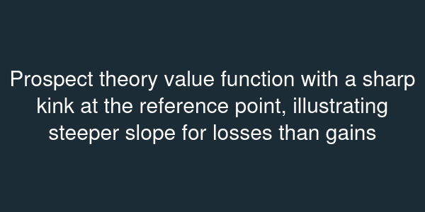
Prospect theory replaces expected utility $U$ with a value function $v(x)$ defined on deviations from a reference point $r$. The typical functional form is

$$v(x) = \begin{cases} (x - r)^\alpha & \text{if } x \geq r, \\ -\lambda (r - x)^\beta & \text{if } x < r, \end{cases}$$

where $\alpha, \beta \in (0, 1]$ capture diminishing sensitivity and $\lambda > 1$ measures loss aversion. Empirical estimates often find $\lambda \approx 2.25$. The kink at $x = r$ represents the discontinuity in slope: $v'(r^-) = \lambda$ while $v'(r^+) = 1$ when $\alpha = \beta = 1$.

Consider a binary gamble: gain $100$ with probability $0.5$ or lose $100$ with probability $0.5$. Under loss aversion with $\lambda = 2$, the subjective value becomes $0.5 \times 100 - 0.5 \times 2 \times 100 = -50$. Even though the expected value is zero, the perceived value is negative, explaining risk aversion for symmetric bets.

Evidence and Applications

In the famous mug experiment, students randomly assigned a coffee mug demanded about $7$ to sell it, while buyers offered only $3$. The endowment effect emerges because sellers treat parting with the mug as a loss relative to ownership. Levitt and List analyzed Chicago taxicab drivers who set daily income targets; they quit early on good days because falling below the target feels like a loss. In finance, the disposition effect shows investors selling winning stocks too early (locking in gains) and holding losers (avoiding losses).

Loss aversion also shapes insurance demand. People overpay for coverage on small deductibles because the potential loss feels catastrophic relative to their reference wealth. Public policy harnesses this by framing incentives as losses: defaulting on health insurance, for instance, triggers a penalty rather than offering a reward for enrollment.

Quantifying Impact

To incorporate loss aversion into models, you adjust payoff matrices. In a labor supply model, the worker chooses hours $h$ to maximize $v(w h - T) - C(h)$, where $T$ is a reference income target. If wages fall short, the marginal disutility of reducing hours is scaled by $\lambda$, producing backward-bending labor supply at targets. In asset pricing, the equilibrium condition becomes $E[\phi R] = 1$ where $\phi$ is the stochastic discount factor incorporating loss-averse preferences; this can explain excess returns because investors demand a premium for bearing downside risk.

Further Reading

• Prospect Theory: An Analysis of Decision under Risk
• Camerer: Prospect Theory in the Wild
• Genesove and Mayer on Loss Aversion in Housing