Expected Utility Theory

Essential Questions

• How does expected utility summarize risky choices into a single number?
• What role do concavity and risk aversion play in the model?
• Which empirical puzzles forced economists to move beyond expected utility?

Overview

A mutual fund asks you to help design client questionnaires that measure risk tolerance. Expected utility theory promises a clean translation from coin flips to calculus: multiply each payoff by its probability, apply a concave utility function, and choose the option with the highest expected value. Yet when you run pilot surveys, people accept gambles that violate the very axioms you used to model them. Understanding both the power and the limits of expected utility is essential.

In this lesson, you will derive the model formally, visualize how curvature captures risk preferences, and dissect paradoxes like Allais and Ellsberg that shook the paradigm. You will see how these contradictions opened the door to prospect theory.

Calculus of Risk

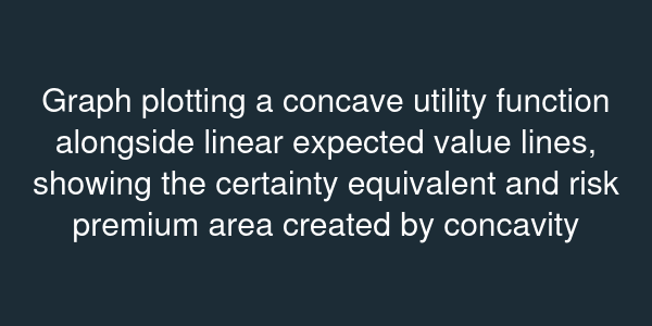
Expected utility theory represents a lottery $L = \{(x_i, p_i)\}_{i=1}^n$ with the number $U(L) = \sum_{i=1}^n p_i u(x_i)$. Risk aversion emerges when $u''(x) < 0$. Consider $u(x) = \sqrt{x}$. For a gamble paying $100$ with probability $0.5$ and $0$ otherwise, $U(L) = 0.5 \sqrt{100} + 0.5 \sqrt{0} = 5$. The certainty equivalent $c$ solves $u(c) = 5$, so $c = 25$, far below the expected value of $50$. The Arrow-Pratt coefficient of absolute risk aversion is $A(x) = -u''(x)/u'(x)$; with $u(x)=\sqrt{x}$, $A(x)=1/(2x)$, shrinking as wealth grows.

When facing continuous distributions, you integrate. If returns follow a lognormal distribution with density $f(r)$, expected utility becomes $\int u(w_0 (1 + r)) f(r) \, dr$. Taking the derivative with respect to portfolio share $\alpha$ and setting to zero gives the first-order condition $\int u'(w_0(1+r(\alpha))) r_i f(r) \, dr = 0$, the canonical asset allocation equation.

Paradoxes and Evidence

Maurice Allais demonstrated that people violate the independence axiom. In his experiment, Option 1 offered a certain $1$ million. Option 2 offered an $89\%$ chance of $1$ million, a $10\%$ chance of $5$ million, and a $1\%$ chance of $0$. Most chose the certainty in the first question but switched to the riskier prospect in a second question where all probabilities were scaled down. Expected utility requires consistent choices under proportional probability shifts; the data say otherwise.

Daniel Ellsberg added ambiguity to the mix. Participants saw an urn with $30$ red balls and $60$ balls that were either black or yellow in unknown proportions. Many preferred a bet on red over black, but also preferred a bet on yellow over red in a second setup—an impossibility under expected utility. Ambiguity aversion suggests that people treat unknown probabilities differently from known risks, a feature missing from the classical model.

Beyond Expected Utility

Economists responded with models like rank-dependent utility, which distorts probabilities, and prospect theory, which introduces reference points and loss aversion. Nevertheless, expected utility remains a benchmark for pricing insurance, evaluating investments, and designing public policy. By mastering its structure, you can specify exactly which axiom a behavioral pattern breaks and choose the right extension.

Further Reading

• Arrow's Essays in the Theory of Risk-Bearing
• Allais Paradox Original Paper
• Ellsberg's Ambiguity and the Savage Axioms