Time Preferences

Essential Questions

• How does exponential discounting translate future dollars into today's value?
• Why does the discount factor imply dynamically consistent planning?
• Where do real people depart from exponential patience?

Overview

You are helping a city design a climate investment plan. The finance team uses net present value to evaluate a flood barrier: discount future benefits, compare to the upfront cost, and make the call. Yet community meetings reveal impatience. Residents demand immediate relief payments even if delaying earns higher interest. Understanding time preferences lets you bridge textbook finance and human behavior.

This lesson takes you through exponential discounting, the calculus behind present value, and the behavioral evidence that points toward time inconsistency. You will compute present values, graph discount factors, and consider policies that confront impatience.

Mechanics of Exponential Discounting

In standard models, future utility is discounted by $\delta^t$ for period $t$. Suppose consumption in period $t$ yields utility $u(c_t)$. The planner maximizes $\sum_{t=0}^{T} \delta^t u(c_t)$ subject to an intertemporal budget constraint $\sum_{t=0}^T \frac{c_t}{(1+r)^t} = W$. Optimality leads to the Euler equation $u'(c_t) = \delta (1 + r) u'(c_{t+1})$, which equates marginal utilities across time adjusted for interest. With CRRA utility $u(c) = c^{1-\gamma}/(1-\gamma)$, this becomes $c_{t+1} = c_t [\delta (1+r)]^{1/\gamma}$, highlighting how growth in consumption depends on patience $\delta$ and the interest rate.

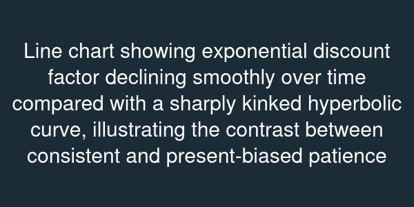
Present value calculations follow: a benefit of $B$ arriving in $10$ years discounted at rate $r$ has present value $PV = \frac{B}{(1+r)^{10}}$. Plotting $\delta^t$ on a semi-log scale yields a straight line, signifying consistent proportional decay.

Evidence of Time Inconsistency

Experiments by David Laibson and others revealed "present bias": people demand far higher compensation to delay a reward from today to tomorrow than from 30 to 31 days. In one study, participants chose between $50$ today or $60$ in a month; most took the immediate cash. When asked between $50$ in six months or $60$ in seven months, the majority waited. Exponential discounting cannot produce this reversal because the ratio $\delta^{t}/\delta^{t+1}=\delta$ is constant.

Field data echo the lab. Savings programs see high enrollment but low continuation. Gym memberships are purchased in January, then neglected. Governments confront similar impatience when designing carbon taxes whose benefits arrive decades later.

Bridging to Behavioral Models

Recognizing the limitations of exponential discounting sets the stage for hyperbolic models where discount factors decline steeply at first and then flatten. Policymakers respond with commitment devices: automatic savings escalators, penalties for early withdrawal, or reward schedules that front-load feedback. As you move into Unit 2, you will see how modifying the objective function with parameters like $\beta$ and $\delta$ captures the observed impatience without discarding the analytical clarity of present value calculus.

Further Reading

• Paul Samuelson's Discounted Utility Model
• Laibson's Golden Eggs and Hyperbolic Discounting
• Climate Discounting and the Social Cost of Carbon